Docker hands-on exercises
Use case 1: Deploy a custom Docker image
- Download the sample code from https://github.com/Azure-Samples/docker-django-webapp-linux.git
- Build the image using the Dockerfile in that repo using
docker buildcommand - Run an instance from that image
- Verify the web app and container are functioning correctly
Use case 2: Simple Bioinformatics example
Let’s say if you find a cool tool/software and want to run it on your computer and as we found out in the morning session, it’s not always easy to install the tool onto your computer or on a server natively. Since this workshop is about containers, let’s containerize this tool.
For this simple hands-on exercise, let’s containerize fastqe tool - https://github.com/lonsbio/fastqe. For those of you who are not from Bioinformatics, this tool generates read one or more FASTQ files, then it will compute quality stats for each file and print those stats as emoji… for some reason.
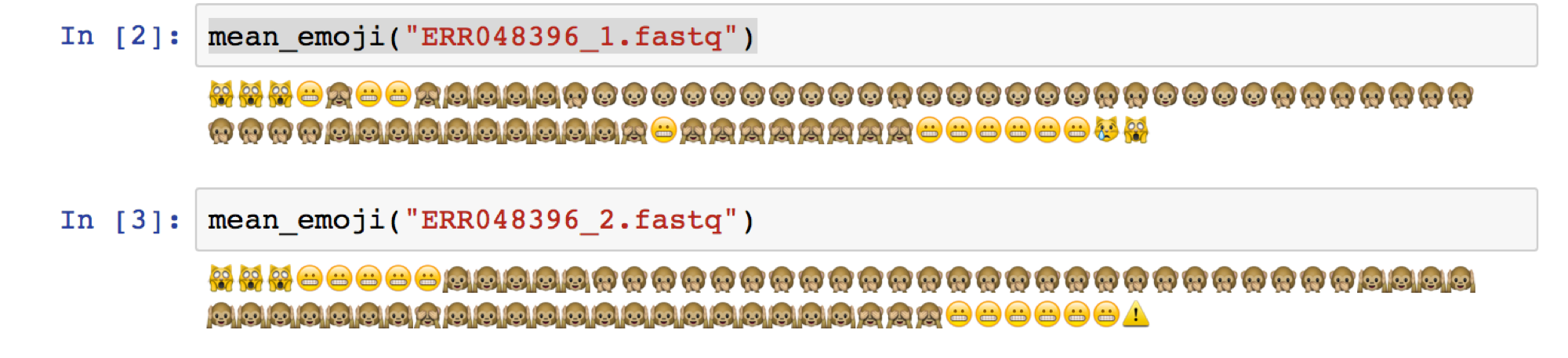
Given a fastq file in Illumina 1.8+/Sanger format, calculate the mean (rounded) score for each position and print a corresponding emoji!
Tip
Natively you would install this tool like pip install fastqe. Now think of how you can dockerize this with appropriate base image and dependencies
After dockerizing the tool, for this exercise we don’t have to bind mount the volume but just print the fastqe help and make sure that it is actually working.
Tip
Natively you would print the help of the tool as fastqe -h
1. Data Management Hands-on
Form the “Introduction to Docker” session this morning, we learned that a running Docker container is an isolated environment created from a Docker image. This means, although it is possible to store data within the “writable layer” of a container, there are some limitations:
- The data doesn’t persist when that container is no longer running, and it can be difficult to get the data out of the container if another process needs it.
- A container’s writable layer is tightly coupled to the host machine where the container is running. You can’t easily move the data somewhere else.
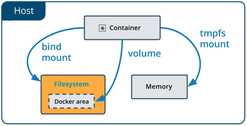
Docker offers three different ways to mount data into a container from the Docker host: volumes, bind mounts, or tmpfs volumes. For simplicity, we will only use bind mounts in our hands-on session, even though volumes is the more powerful and usable option for most use cases.
1.1 Bind mounts
Bind mounts: When you use a bind mount, a file or directory on the host machine is mounted into a container.
Warning
A side effect of using bind mounts, for better or for worse, is that you can change the host filesystem via processes running in a container, including creating, modifying, or deleting important system files or directories. This is a powerful ability which can have security implications, including impacting non-Docker processes on the host system.
If you use --mount to bind-mount a file or directory that does not yet exist on the Docker host, Docker does not automatically create it for you, but generates an error.
Let’s clone a git repository to obtain our data sets:
$ git clone https://github.com/CyVerse-learning-materials/ccw-2019-astro.git
We can cd into the HOPS work directory, and mount it to /root as we launch the eventhorizontelescope/hops container:
$ cd ccw-2019-astro/hops
$ ls
1234
$ docker run -it --rm --name hops -v $PWD:/root eventhorizontelescope/hops
Setup HOPS v3.19 with HOPS_ROOT=/root for x86_64-3.19
You will start at the /root work directory and the host data 1234 is available in it:
$ pwd
/root
$ ls
1234
You can open another terminal and use docker inspect hops | grep -A9 Mounts to verify that the bind mount was created correctly. Looking for the “Mounts” section,
$ docker inspect hops | grep -A9 Mounts
"Mounts": [
    {
        "Type": "bind",
        "Source": "/Users/ckchan/ccw-2019-astro/hops",
        "Destination": "/root",
        "Mode": "",
        "RW": true,
        "Propagation": "rprivate"
    }
],
This shows that the mount is a bind mount with correct source and target. It also shows that the mount is read-write, and that the propagation is set to rprivate.
Use case 1: Processing VLBI data with HOPS in Docker
HOPS stands for the Haystack Observatory Postprocessing System. It is a standard data analysis tool in Very-long-baseline interferometry (VLBI). HOPS has a long history and it depends on legacy libraries. This makes it difficult to compile on modern Unix/Linux systems. Nevertheless, with Docker, you have already launched a HOPS envirnment that you can analysis VLBI data!
The most basic step in analysis VLBI is called “fringe fitting”, which we will perform in the running HOPS container by
$ ls 1234/No0055/
3C279.zxxerd  L..zxxerd  LL..zxxerd  LW..zxxerd  W..zxxerd  WW..zxxerd
$ fourfit 1234
fourfit: Warning: No valid data for this pass for pol 2
fourfit: Warning: No valid data for this pass for pol 3
$ ls 1234/No0055/
3C279.zxxerd  LL..zxxerd     LL.B.2.zxxerd  LW.B.3.zxxerd  W..zxxerd   WW.B.5.zxxerd
L..zxxerd     LL.B.1.zxxerd  LW..zxxerd     LW.B.4.zxxerd  WW..zxxerd
fourfit reads in the correlated data and create the so called “fringe files”. The warnings are normal because there are missing polarizations in the data. In order to see the result of the fringe fitting, you can use fplot:
$ fplot -d %04d.ps 1234
$ ls
0000.ps  0001.ps  0002.ps  0003.ps  0004.ps  1234
Congratulations! You just created 4 fringe plots that show all important information of the VLBI experiment! Now you can exit your HOPS container and open them on your host machine.
2. Jupyter Notebook Hands-on
Mounting a host directory is one way to make a container connect with the outside work. Another possible is through network by exposing a port.
Use case 2: Processing Galaxy Simulation with Jupyter in Docker
In this second hands-on, we will use Docker to run a “ready to go” Jupyter notebook in a container. We will expose the port 8888 from the container to the localhost so that you can connect to the notebook.
Inside the ccw-2019-astro git repository that you downloaded earlier, there is a sample Galaxy simulation:
    $ pwd
    /Users/ckchan/ccw-2019-astro/hops
    $ cd ../galaxy/
    $ pwd
    /Users/ckchan/ccw-2019-astro/galaxy

    # Specify the uid of the jovyan user.  Useful to mount host volumes with specific file ownership.  For this option to take effect, you must run the container with --user root

    $ docker run -it --rm -v $PWD:/home/jovyan/work -p 8888:8888 -e NB_UID=$(id -u) --user root astrocontainers/jupyter
    Set username to: jovyan
    usermod: no changes
    Set jovyan UID to: 1329
    Executing the command: jupyter notebook
    [I 23:36:09.446 NotebookApp] Writing notebook server cookie secret to /home/jovyan/.local/share/jupyter/runtime/notebook_cookie_secret
    [W 23:36:09.686 NotebookApp] WARNING: The notebook server is listening on all IP addresses and not using encryption. This is not recommended.
    [I 23:36:09.722 NotebookApp] JupyterLab beta preview extension loaded from /opt/conda/lib/python3.6/site-packages/jupyterlab
    [I 23:36:09.722 NotebookApp] JupyterLab application directory is /opt/conda/share/jupyter/lab
    [I 23:36:09.730 NotebookApp] Serving notebooks from local directory: /home/jovyan
    [I 23:36:09.730 NotebookApp] 0 active kernels
    [I 23:36:09.730 NotebookApp] The Jupyter Notebook is running at:
    [I 23:36:09.730 NotebookApp] http://[all ip addresses on your system]:8888/?token=a81dbeec92b286df393bb484fdf53efffab410fd64ec8702
    [I 23:36:09.730 NotebookApp] Use Control-C to stop this server and shut down all kernels (twice to skip confirmation).
    [C 23:36:09.731 NotebookApp]
    Copy/paste this URL into your browser when you connect for the first time,
to login with a token:
    http://localhost:8888/?token=dfb50de6c1da091fd62336ac52cdb88de5fe339eb0faf478
The last line is a URL that we need to copy and paste into our browser to access our new Jupyter Notebook:
http://localhost:8888/?token=dfb50de6c1da091fd62336ac52cdb88de5fe339eb0faf478
Warning
Do not copy and paste the above URL in your browser as this URL is specific to my environment.
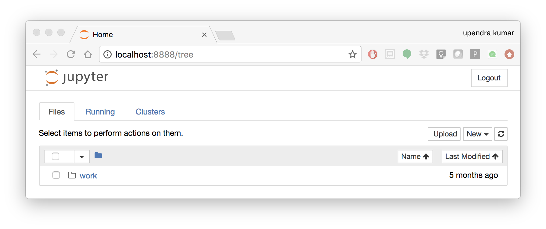
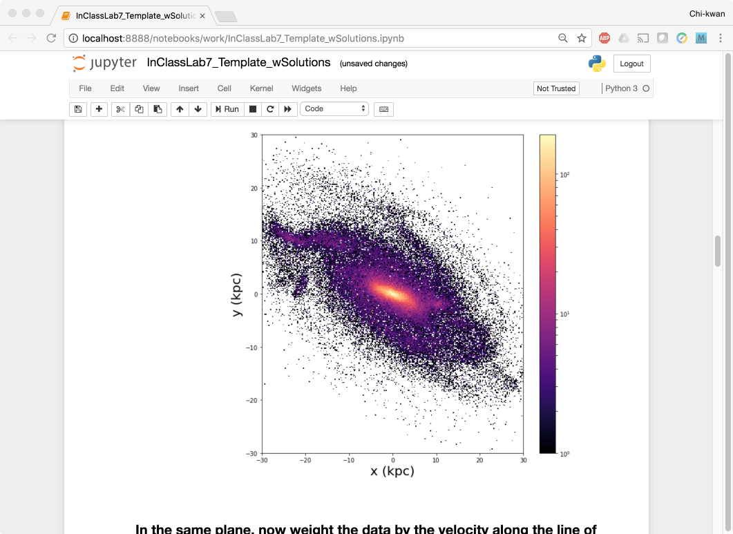
You should be greeted by your own containerised Jupyter service! Now open galaxy/InClassLab7_Template_wSolutions.ipynb and try analysis a Galaxy simulation!
To shut down the container, simply hit Ctrl-C in the terminal/command prompt twice. Your work will all be saved on your actual machine in the path we set in our Docker compose file. And there you have it—a quick and easy way to start using Jupyter notebooks with the magic of Docker.